
Hereafter, we discuss so-called "triangular plots"; this means relationship between the absolute magnitude H and the (proper) orbital elements a, e, sin i. We compare the results of our numerical simulation with the observed distribution of Eos family asteroids (their proper elements are taken from AstDys catalogue; membership identifications are done by means of HCM method). Moreover, we briefly comment on possible dynamical processes, which might have affected the overall shape of Eos family, with emphasis to what could be learnt from these "triangular plots" (remember that each asteroid family seem to be unique and particular with this respect!).
The main page on asteroids families, with a detailed description of the model, is available here.
Initial conditions of the numerical simulations:
NTP = 210; osculating elements, thermal parameters: radii from 1.0 upto 32.3 km (see data file), bulk density 2500 km/m3, surface density 1500 km/m3, thermal conductivity 0.001 W/K/m, thermal capacity 680 W/kg/K, albedo 0.10, infrared emissivity 0.90, random rotation periods between 4 - 12 hr, random (and fixed) spin axes orientations.
Please notice, that the initial dispersion in a, e, sin i space does NOT resemble the current, observed shape of the Eos family. Mainly, we did not took into account the dependence of the dispersion on asteroids' radii (with larger fragments closer to the family barycenter and smaller ones farther). This could be clearly seen at Figure 1. This may seem as a drawback, but note that big bodies basically did not move during the simulation, so that putting them more tightly around the center of the family they would stay there.
List of figures:
See also:
| initial state | after 600 Myr | |
| H(a) |  |
 |
| H(e) |  |
 |
| H(sin i) |  |
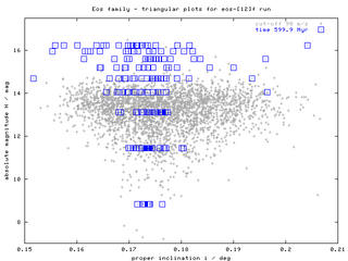 |
Figure 1 - "Triangular plots", sequences of H(a), H(e), H(sin i) plots for times 2.5 Myr and 600 Myr. According to these figures, the initial "box-like" structure of the swarm slowly disperses (in all the elements) and forms something, which can roughly resemble "triangular" cloud of observed asteroids. The data (proper elements of our bodies) are avaiable here. Click on the left images to obtain a whole sequence/animation with time-step 100 Myr.
The smallest (yet unobservable) asteroids (H > 16 mag) might be after 2 Gyr evolution even strongly depleted from this family (by their interactions with J9/4, J7/3 and J11/5 resonances). This certainly depends on the timescale of spin axis reorientations (which might be affected by collisions, YORP effect and possible spin-orbital resonances). Note also, that the extension of the corresponding "triangle" of the observed family depends on the HCM cutoff velocity as we shall discuss below.
Figure 2 - Here is a plot of the proper a(t) and dispersion of semimajor axes sigmaa during our 600 Myr simulation. Note the "traffic" across the J9/4 resonance and how only a fraction of asteroids get through it.
 |
 |
Figure 3 and 4 - Proper (a, e) and (a, i) plots with evolutionary paths of "synthetic" bodies and comparison with family members in the background (at the HCM cut-off velocity equal to 90 m/s).
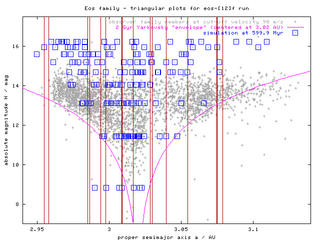
Figure 5 - H(a) plot of observed Eos family members at three different cut-off velocities (60, 80 and 90 m/s) and also including resonance borders. The marked width of resonances is calculated for the mean eccentricity of the Eos family (ie. resonances could be narrower/wider for asteroids with lower/higher eccentricities).
There is a significant number of asteroids behind the right branch of "Yarkovsky envelope". They cannot reach this location from the family center (at 3.02 AU) within 2 Gyr by Yarkovsky drift (even in case of most favorable spin axis orientation). Certainly, the furthermost may be interlopers in the family: we actually already known about few of them aaand if everything goes well during this spring, we should have a much clearer idea about these objects "far from the Yarko envelope".
Additionally the drift could be effectively speeded up by jumping through resonances (the widest "en route" are J9/4, J11/5 and 3J-2S-1). Notice that behind the J11/5 resonance the overlap is even more increased (upto 0.02 AU), which could possibly support this hypothesis. However, the sum of effective widths of all these resonances seem to be smaller than 0.02 AU, and this would be the maximum gain as compared to the Yarko drift.
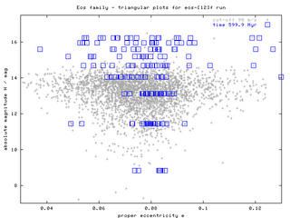
Figure 6 - H(e) plot at the three cut-offs. Only at 90 m/s cut-off we include both groups of low and high eccentricity bodies, thus we use this cut-off in the following plots.
Figure 7 - H(e) plot with asteroids on right/left side of 9:4 mean motion resonance with Jupiter. Practically all bodies with eccentricities higher than 0.105 - and forming thus the bulk of the "right wing" in the H(e) triangle at higher HCM cutoffs - are also located on the right side of J9/4 resonace, which may indicate, that crossing through J9/4 is responsible for the eccentricity increase.
Figure 8 - H(sin i) plot displaying bodies on the left/right side of J9/4 resonance. Here we do not see a strong difference between inclination distributions (as J9/4 does NOT strongly affect the value of inclination).
Figure 9 - H(e) distribution of asteroids in z1 secular resonance (with |z1 frequency| < 1"). Most of asteroids with e < 0.047 are likely to be affected by z1 resonance; they could reach this low-eccentricity region by "sliding along" the resonance borders, while drifting by Yarkovsky effect.
Figure 10 - H(sin i) plot with asteroids in z1 resonance. The triangular shape does not seem to be somewhat correlated with the distribution of these asteroids.