
Introduction. Here we attempt to address the origin of asteroids, which are located inside the 2:1 mean motion resonance with Jupiter and reside on quasi-stable orbits with lifetimes on the time-scale several hundred Myr (that is the case of ~20 observed asteroids, so called Zhongguos). We are testing the hypothesis, that bodies originate in the Themis family, which is close to the lower edge of the 2:1, with the Yarkovsky effect driving them onto their present stable location. We shall see that the result is basically negative, and together with our belief that the initial velocites of the Themis members were not large enough to inplace Zhongguos directly, this would suggest that Zhongguos are unrelated to the Themis family (possibly a residual population initially formed in the J2/1 resonance?).
Initial conditions of numeric simulations. 500 TPs (250 of them were processed upto now), only 4 outer planets (!), obliquity gamma = 45° - ie. particles drift outwards, head to the 2:1 mean motion resonance with Jupiter. Distribution of a, e, i elements roughly resembles the part of Themis family closer to the 2:1 resonance (see Fig. 1).
As far as the size distribution, thermal parameters and rotational
states of the TPs are concerned, we chose the same as those selected for the Themis
family itself (ie. runs themis-[12]).
Radii are ranging from 1 km upto 1.7 km (250 TPs, run
r21-3b - these results are presented below!)
and from 1.7 to 55 km (also 250 TPs, the run is refered
as r21-3a and is not yet processed).
Bulk and surface density is 1300 kg/m3,
thermal conductivity 0.01 W/m/K,
thermal capacity 680 W/kg/K
albedo 0.02,
and infrared emissivity 0.95.
Rotational axes are oriented randomly and isotropically in space.
Rotational periods are equally distributed between 4 and 12 hours.
2DO: process the rest 250 TPs from the r21-3a run
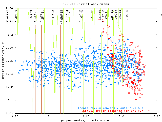
Fig. 1 - Initial proper elements (a, e) of 250 TPs and comparison with the observed Themis family members, identified by the HCM method at 90 m/s cutoff velocity.
Averaging technique, resonant elements. Outside the resonance we usually use on-line filtering based on on a sequence of convolution filters (so-called Kaiser windows), in this case we used initial sampling 1 yr and sequence of four filters AAAB with corresponding decimation factors 10 10 5 3, resulting in output every 1500 yr, which is free of periods shorter than approx. 1000 yr. After that we calculate "proper" elements by a running window method, the window is typically 5 Myr wide). Additionally, we store the osculating elements, but only every 10 kyr (see below, that this long sampling of the osculating elements causes some problems).
The motion inside the 2:1 resonance is dominated by short periodic oscillations of the critical argument libration (approx. 300-400 yr, see spectra below on Fig. 8) of both semimajor axis and eccentricity. Because of the on-line filter, not properly adjusted to the 2/1 dynamics (the shame goes to DV), the structure of the resonance becomes completely smoothed by the averaging described above, so we have to use a slightly different approach (actually, somewhat adhoc solution). To keep the information on the amplitude of (coupled) a, e oscillations, we used a running minimum (or maximum) filter, ie. we restarted the integration (from the osculating elements stored every 10 kyr), ran for 500 yr (what is definitely longer than one oscillation period) and kept only one datum from this short run - that one, where a is minimal.
Unfortunately, aliasing problem could arise from the fact, that medium-period oscillations (approx. 20 kyr) are undersampled. (This is addressed below, see Fig. 9 and explanation in text.) To remove these oscillations completely, we finally applied 1 Myr running window, certainly a method that partially corrupts the fine details of the in-resonance dynamics. The orbital elements computed by the described method are hereafter called "resonant", simply because we use them for the motin inside the 2/1 resonance.
David, Morby, etc.: could you please suggest a better method of handling our previour mistake of too much "filtering" and too sparse sampling of the osculating elements?
Resonant (a, e) plots and "transport maps" of the 2:1 resonance. We call the colour coded (a, e) plot as "transport maps" - see Fig. 2 for explanation.
 |
 |
Fig. 2 -
(a) Resonant (a, e) plot for the r21-3b
simulation and all 250 TPs. You can compare it with usual
proper (a, e) plot,
where all particles are located in the middle of the 2:1
resonance and consequently no structures could be seen.
(b) (a, e) plot with the same scale, but the colour
coding of rectangular cells displays the total number of test particles, which
were located inside the cell, summed over all time steps; in practice
this means 20 kyr, namely the 1 Myr smoothing window moved by
20 kyr.
One can also imagine it as a 3-dimensional cube (a, e,
t) projected on the (a, e) plane
with the colour coded density of points:
blue denotes stable regions (occupied by many
asteroids for considerably long time), whilst there is little points in the
red cells (and no points in white). Lower number
of recorded asteroids in a cell means
either little TPs reach this location or it is an dynamically unstable
region, where TPs reside for only a short time.

Fig. 3 - (a, sin i) plot with the same colour coding as in Fig. 2.
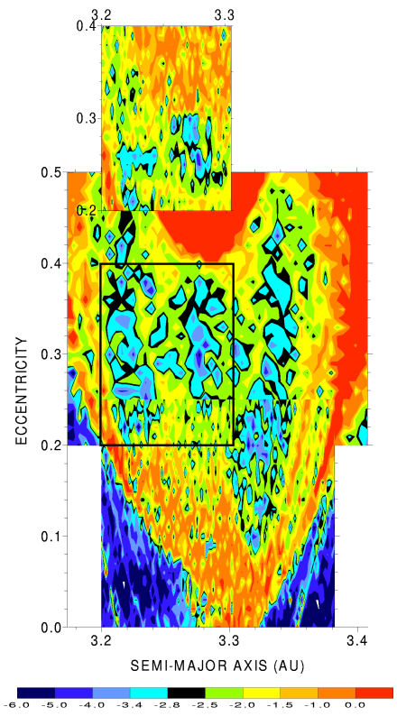
A comparison of the chaotic diffusion rates and our "transport map" is possible on Fig. 4. The well known structures from Fig. 4a (such as fast diffusion on separatrices or stable islands inside the resonance) are also visible on Fig. 4b.
In spite of that, we do not observe any long term (>100 Myr) captures of our TPs in the 2/1 resonance, resembling Zhongguos orbits (see resonant a(t) plot). Moreover, the capture periods might be even shorter, if we include inner planets in the simulation.
(Rem. Mira is going to process real Zhongguos using his software and plot them in 4b for sake of comparison; he also wants to plot distribution of the residence time in 2/1 for TPs.)
 |
 |
Fig. 4b -
(a) A chart of chaotic diffusion in the J2/1 resonance. Red color represents
high values of log10|delta dvarpi/dt|,
while blue denotes slow diffusion rates.
(Adapted from Nesvorny and Ferraz-Mello 1997.)
(b) (a, e) plot for the r21-3 simulation,
with similar scale and colour palette as in the previous case (a).
The colour coding of rectangular cells displays the total number of test
particles, which were located inside the cell, summed over the whole
time span of the integration.
Yarkovsky driven diffusion through the 2:1 resonance. Four particles (out of 250, ie. 1.6 %) crossed the 2:1 resonance (Fig. 5). However, remember the inner planets were missing in this simulation, and perihelia of 3 TPs reached Mars crossing region (Fig. 6); some of them might be eliminated during this period. Thus we can conclude, that approx. 1 % of Themis asteroids (in the size range 2 - 3.5 km) might be able to cross the 2:1 resonance.
Fig. 5 - Proper (a, e) plot for particles 4, 141, 179 and 236.
Fig. 6 - Perihelia of 4 test particles, which finally crossed the 2:1 resonance. The capture periods span from 0 Myr (TP no. 4, see below) to 40 Myr.
Fourier analysis of osculating a(t), e(t) signals for TP no. 4.
We selected one test particle for the detailed inspection of motions
inside the 2:1 resonance. For this purpose we re-calculated (and saved
osculating elements) of TP no. 4 (from r21-3b set)
between 300 and 300.5 Myr.
(Do not be surprised, that TP "jumped" over the resonance very quickly
in the original integration, while in this short run, it stayed
inside until the end, ie. much longer time. It is caused by the
chaotic dynamics in the resonance; this calculation was also
performed on a different computer than previously.)
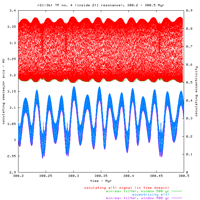
Fig. 7 - Fourier transform of the a(t) and e(t) signals, both osculating and filtered; this is the low-frequency part, 10 kyr corresponds to about 130 ''/yr.
The Fourier transform of a(t) signal (Fig. 8) reveals two significant frequencies - approx. 350 yr and 21.5 kyr. The short-periodic oscillation (J2/1 librations) could be removed by the previously described procedure. Unfortunately, the long-periodic oscillations are slightly undersampled because of our (bad) choice of storing the osculating elements only every 10 kyr. It leads to an aliasing in the frequency domain. According to the sampling theorem: the sampling rate s should be such that all frequencies higher than s/2 must not be present in the sampled signal. This is not true in our case (the necessary sampling rate is approx. 7 kyr). The output signal is thus degraded. This is why we were forced to apply the "artificial" smoothing by the 1 Myr running window, removing thus the intermediate-period oscillations in the resonance.
It seems to us, that the only solution how to remove 20 kyr oscillations in a more sophisticated way, and than possibly resolve finer structures of the 2:1 resonance, is to re-done the simulation with a different output rate setup. IS THERE ANY OTHER HELP?
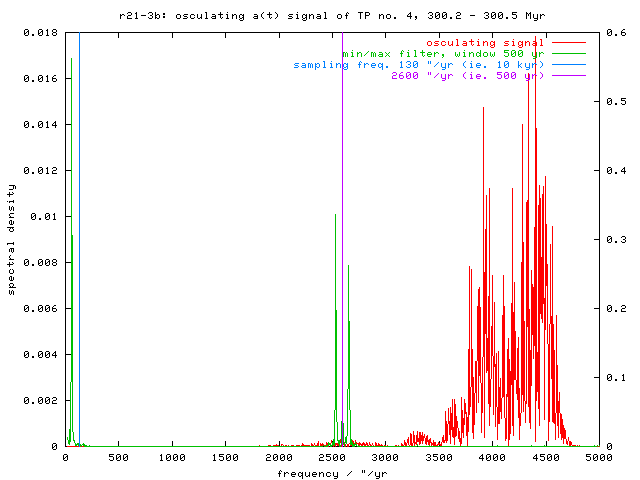
Fig. 8 - Frequency domain of a(t) signal (its part from 300.2 to 300.5 Myr). The spectrum of osculating element is red, the spectrum of signal filtered by above described "minimum a" filter is green. The peak 60 "/yr is also present in the osculating data, but its spectral density is relatively very low (10-5) to the short-periodic signal - that is the reason, why it is not visible on this plot. The peak around 2500 "/yr in filtered signal (ie. sampling frequency of the transformed signal) is an artefact of the FT and it makes no odds.
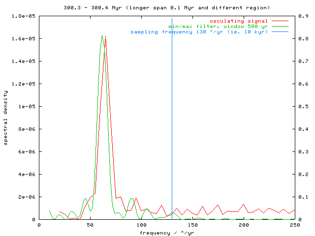
Fig. 9 - Detail of the low frequency region; in this figure the a(t) data are taken only from interval 300.3 to 300.4 Myr. The vertical line denotes the sampling frequency s (130 "/yr, the corresponding period 10 kyr). It is evident, that signal has significant power well beyond s/2, what leads to an aliasing.
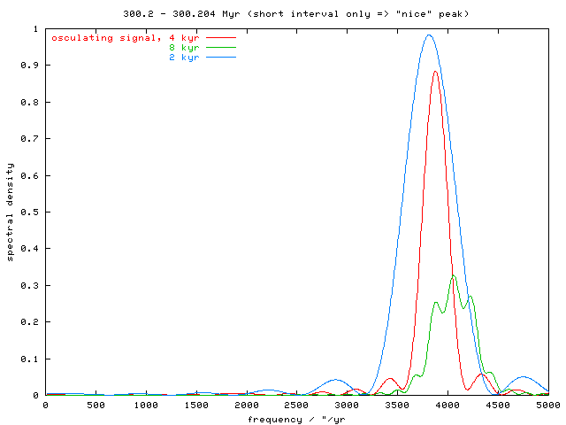
Fig. 10 - Fourier analysis of short (4 kyr) fragment of osculating a(t) signal shows prominent frequency 3800 "/yr (ie. period 330 yr); long period component naturally vanishes. The longer time-span, the more complex is the spectrum.
Fig. 11 - Critical angle of the J2/1 resonance (2lambda-lambda'-varpi; constant in the phase is not cured here). At 300.2 Myr the TP enters the of the resonance (via Yarkovsky drift) and starts to librate.
Stability of orbits inside the 2:1 with/without Yarkovsky effect. This issue was already tested - see this page. We observed no significant change of orbital stability (lifetime) of Griquas and Zhongguos between calculations with and without Yarkovsky effect.