In this work we focus on the unstable population of objects and investigate the hypothesis that they are continously replenished by the Yarkovsky-driven transport from the main-belt zone "below" the resonance. Assuming mean albedo of 0.05, Mira computed the following numbers of currently known objects in the three different 2/1 subpopulations:
|
Population |
Number of |
Number of |
|
Zhongguos |
|
|
|
Griquas |
|
|
|
unstable |
|
|
... and here is the plot of their size distributions:
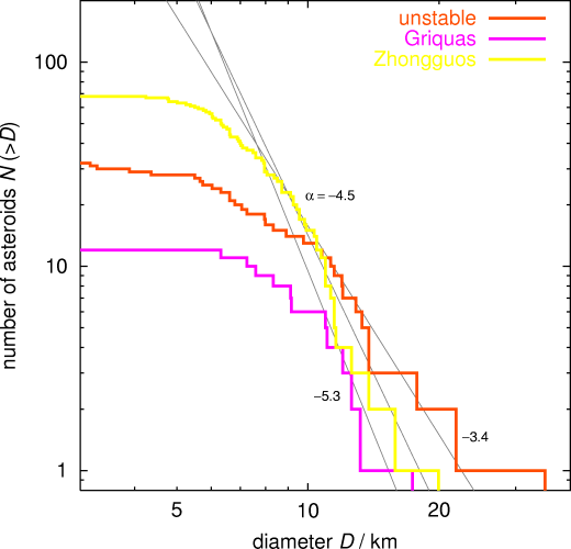
The slopes of SDs were determined by least-square fitting of a linear function in the following intervals of diameter: Zhongguos < 8, 20> km, Griquas <10, 15> km, unstable <10, 15> km. We note that Zhongguos have a pretty steep size distribution (α = -4.5), which make this population distinct from the others. Griquas are few and perhaps it is difficult to say something very reasonable; the unstable asteroids are also few but apparently have a quite shallower size distribution than Zhongguos. Our fitted exponent (α = -3.4) has uncertainty of ~ 0.1, say.
Populations of the guessed source regions.
Our first guess of the source region for unstable asteroids was the Themis family; after all it is the most populous family near the 2/1 resonance and historically it was suggested to be the source of all 2/1 asteroids [Ref]. However, there is no a priori reason to disregard background (non-family) asteroids as a potential source too. In fact, they largely dominate (by a factor of ~ 4) family asteroids! So Mira took a look at the populations there and came with the following results (both Themis and Hygiea were identified by the HCM method and we used 70 m/s as a cut-off velocity):
|
Population |
Number of |
|
Themis |
|
|
Hygiea |
|
|
background |
|
Size distribution of these subpopulations, as determined with a simplified assumption of 0.05 albedo uniformly, are as follows:
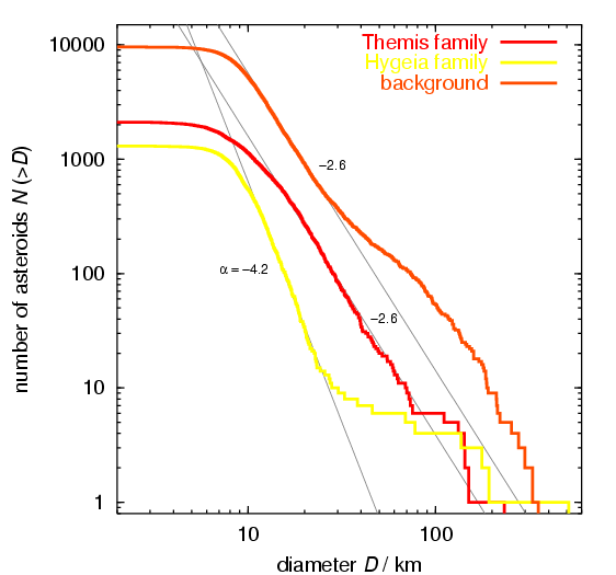
Hence, both Themis and the background populations are matched in the 10 - 50 km range with a power law having exponent of ~ -2.6. The Hygiea is a bit anomalous with a rather steep slope of ~ -4.2 and a number of really large asteroids (with >100 km size); note, however, that Hygiea is just a small population as compared to both Themis and, especially, the background groups. Their pretty shallow distribution does not immediately match distribution of the unstable 2/1 asteroids and it is a challenge of our model to explain this difference in slopes. Obviously, we know that the Yarkovsky effect is size dependent, roughly as 1/(size), so that a difference up to -1 in the two slopes can be explained. Moreover, as in the NEA work [Ref] we expect that at smaller sizes YORP will hinder the Yarkovsky diffusion in the semimajor axis by more frequently reorienting spin axes, and thus a difference little smaller than 1 in the source and unstable asteroids is indeed expected. This issue, together with the absolute number of objects in the populations, is investigated by the semianalytic approach below.
Numerical simulations.
In this part we describe results of numerical simulations we did so far. Their purpose was to see in detail evolutionary paths of orbits pushed by the Yarkovsky effect from the main-belt region below the 2/1 resonance toward it. We are mainly interested in the flow of orbits inside the resonance. We do confirm earlier finding by Roig et al., [Ref] and [Ref], that such Yarkovsky-driven flow towards the resonance cannot place asteroids onto Zhongguo-like or even Griqua-like orbits; the orbits are basically `scattered on the resonance', but still our goal is to see whether such a process is compatible with populating the 2/1 population on unstable orbits. The quantitative issues are investigated below (see Semianalytic steady-state model), while here we mainly want to compare locations of the unstable asteroids inside the resonance and the residence charts corresponding to Yarko-injected orbits into the resonance. We integrate separetely asteroids from three distinct sources: (i) background population, (ii) Themis family, and (iii) Hygiea family. They are characetrized by different pre-resonance value of inclination (mainly) and we wondered if this can somehow modify results; later we shall however see that the differences are not large.
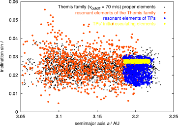
Initial data/population. To that end, we chose a sample of initial orbits and evolve them via direct 1 Gy numerical integration using swift_mvs2_fp_y integrator (Mira's version of swift with the second-order symplectic method and Yarkovsky implemented) with a timestep of 91.3 days (4 outer planets included). The initial positions of 1000 TPs in each population are chosen, so that they satisfy the conditions \sigma=0 and \varpi-\varpi'=0 (see below); this prevents the orbits to fall immediately into the resonance (as they are at `maximum distance' from it) and lets them shortly evolve by the Yarkovsky effect before entering the resonance. The following figures show the initial orbital elements in the (a,e) and (a,sin I) projections for the Themis source:
 |
 |
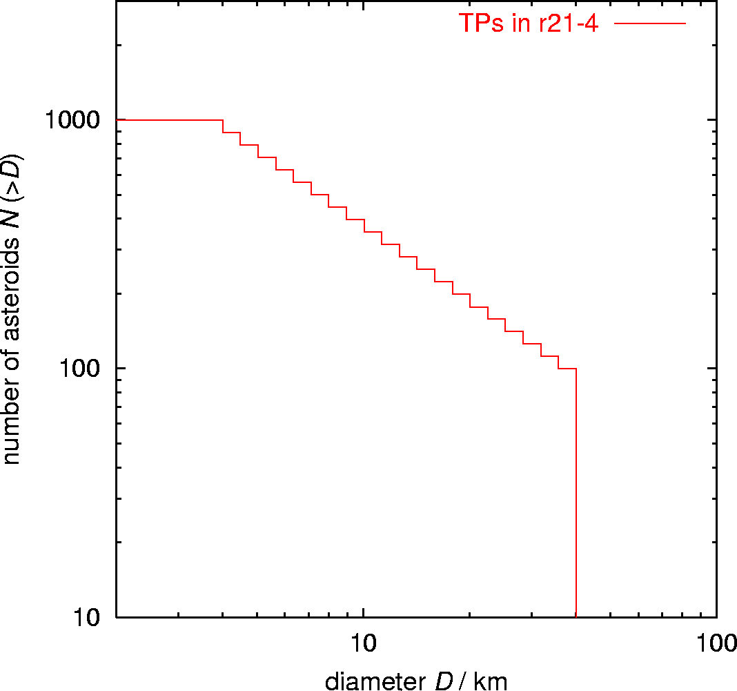
Since the Yarkovsky effect is size-dependent, we integrated bodies of different size: 500TPs were larger than 10 km, and 500 TPs were smaller than 10 km. Here is the cumulative size distribution of the integrated TPs:
We may however say that our results do verify the a priori expected conclusion: the Yark effect determines the rate of transport before entering the resonance, so that smaller asteroids are delivered at a higher pace, but once inside the resonance evolution of asteroids with different sizes is basically the same; the resonant, gravitational dynamics overtakes the Yark effect. So details of the TP size distribution does not really affect conclusions.
Resonant proper elements. The principal advancement as compared to the results presented in Berlin (ACM2002) is Mira's output of the resonant proper elements (instead of just filtered, mean elements). These are discussed in detail by Morby et al. in [Ref], so we give here only a brief outline: once in the resonance, the long-term variations of orbital elements are dominated by:
- the libration cycle of the resonance angle (principal is \sigma=\lambda-2\lambda'-\varpi) with a typical period of 300-400 y, within which semimajor axis and eccentricity, whose coupled angular variables are in \sigma, undergo oscillation between minimum and maximum values, and
- thanks to the long-term variation of Jupiter's eccentricity, there is an overlying oscillation of the semimajor axis and eccentricity with a period of ~ 20 ky and related to a circulation of \varpi-\varpi'.
There are even more subtle variations, affecting inclination too, but for sake of simplicity we use the principal terms described above only (analytical and semianalytical investigations also in Morby's et al. [Ref] and [Ref] and references therein). Hence, we record semimajor axis and eccentricity when (i)\sigma=0, and (ii) \varpi-\varpi'=\pi. At that instant semimajor axis is at a minimum value and eccentricity at a maximum value over the combination of the two cycles. We call these values of semimajor axis and eccentricity resonant proper elements and Mira installed an on-line filter that computes these values. Thanks to chaotic evolution in the resonance, the resonance proper elements are not stable over a very long term and evolve typically toward large values of eccentricity and inclination (Morby and David N. know details of what is going on, secular resonances inside 2/1 MMR etc....). With a high eccentricity value, the orbits are efficiently scattered by Jupiter. A typical integrated orbit looks like on the following figures:
???
|
|
|


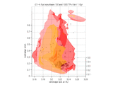
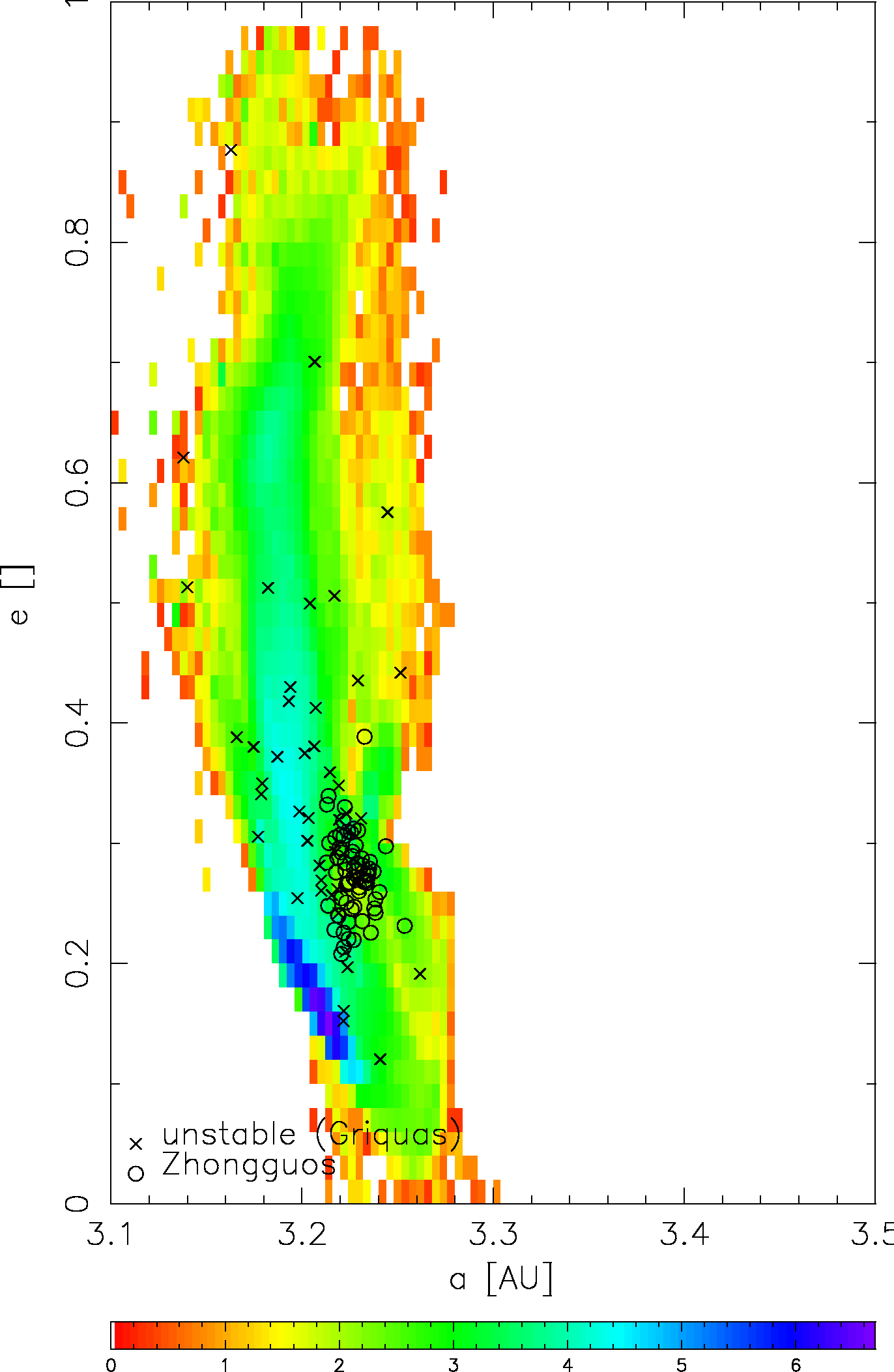
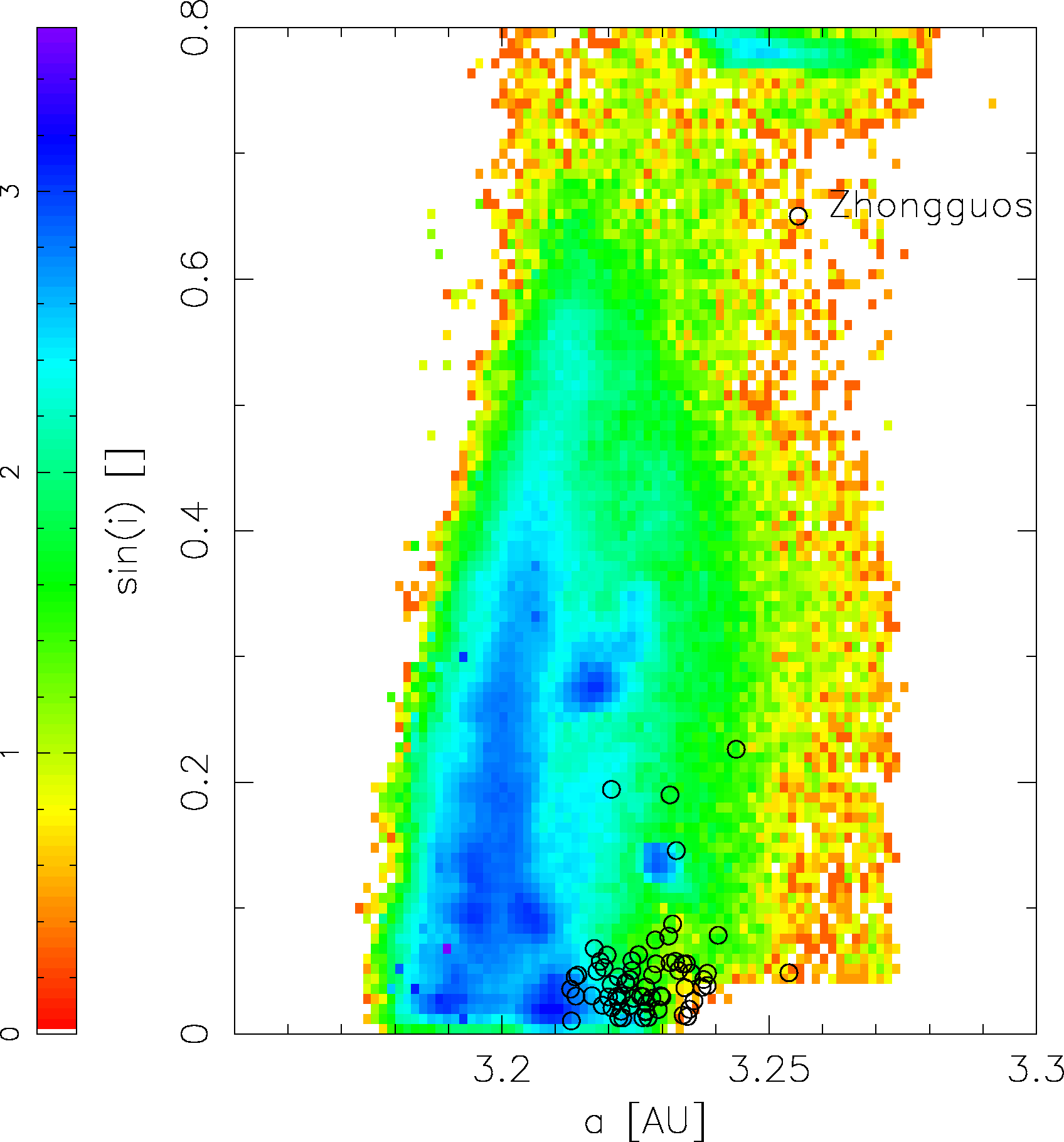
The results of numerical simulations are presented in the form of "transport maps" - i.e. plots of number of TPs, which entered given (a, e, sin(i)) cells during the entire simulation time-span (1 Gyr). Positions of TPs in the resonant (a, e, sin(i)) space were calculated with a time-step of 0.01 Myr. (One TP, which would stay in one cell during the entire simulation, produces a density equal to 100000.) This distribution density of our TPs is to be compared with the observed populations of both stable and unstable asteroids in the J2/1 resonance. We can do it either in various 2-D projections to (a, e) and (a, sin(i) planes or in 3-D views of isosurfaces of the density.
There is a common coding of the asteroid populaions in the following
figures:
circles (o) - stable Zhongguos;
squares - semi-stable Griquas;
crosses (x) - unstable asteroids.
Themis family as a source.
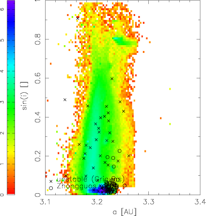
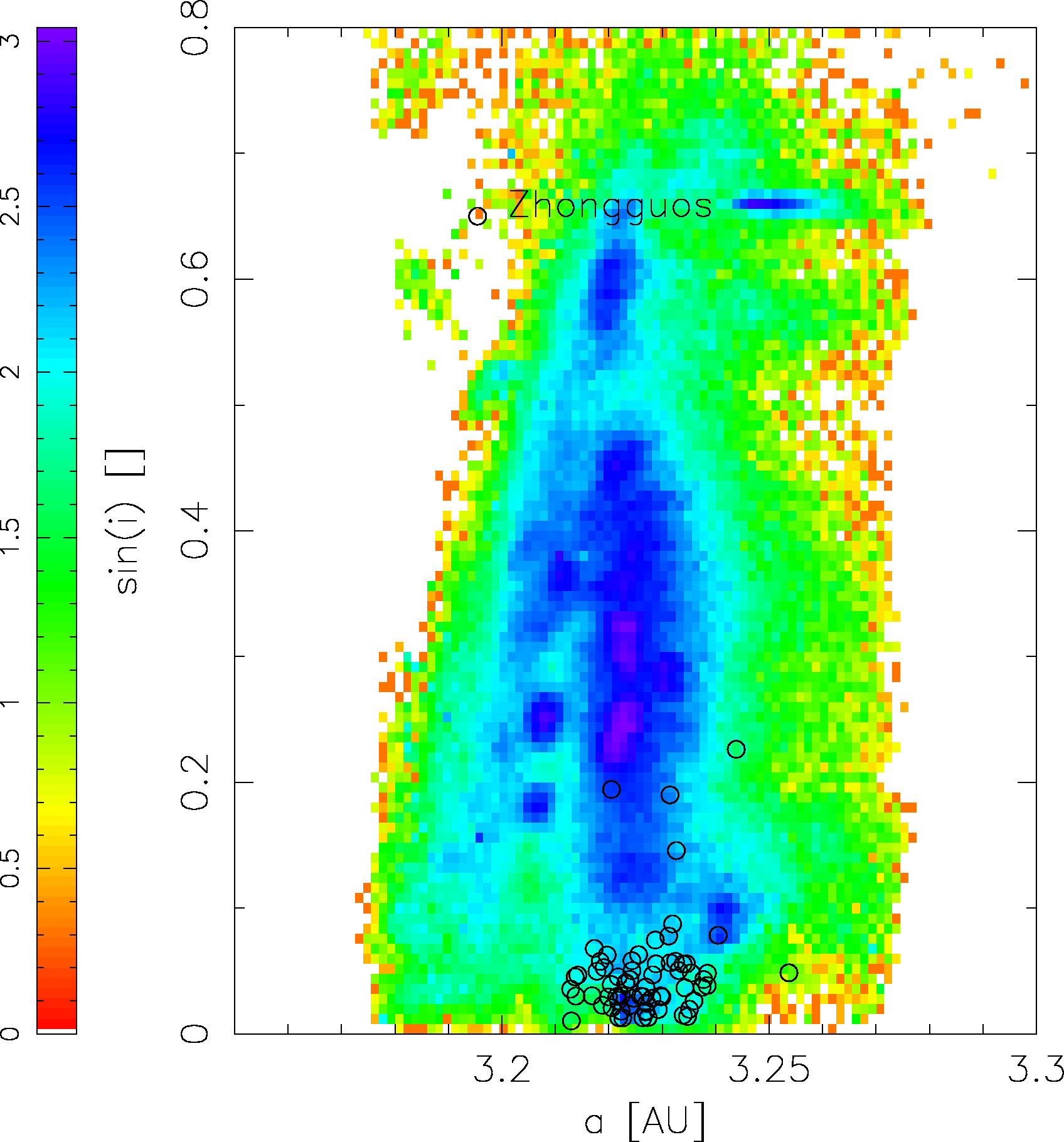
An overall view of the projected (a, e, sin(i)) space with large ranges of the axes is on the two following figures. The logarithm of the density of TPs is colour coded, with blue denoting the highest density and red the lowest. However, the distribution of TPs and observed asteroids cannot be directly compared here, because the projection of the whole sin(i) or e dimension causes that different populations and places of higher density are covered by each other. Moreover, TPs, which did not entered the J2/1 resonance yet, are also visible as a dark-blue patch.
 [ 300 DPI
| EPS ]
[ 300 DPI
| EPS ]
 [ 300 DPI
| EPS ]
[ 300 DPI
| EPS ]
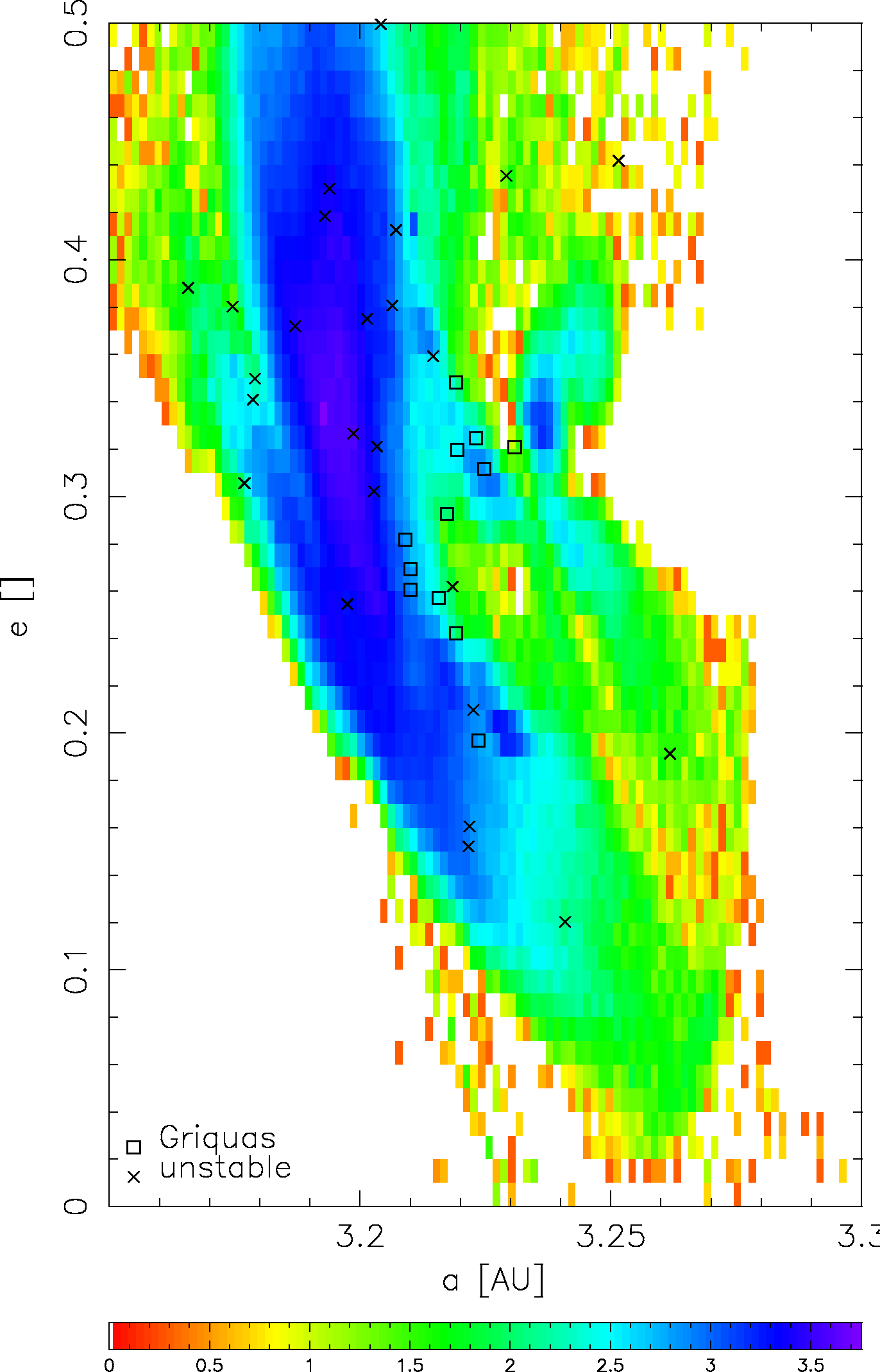
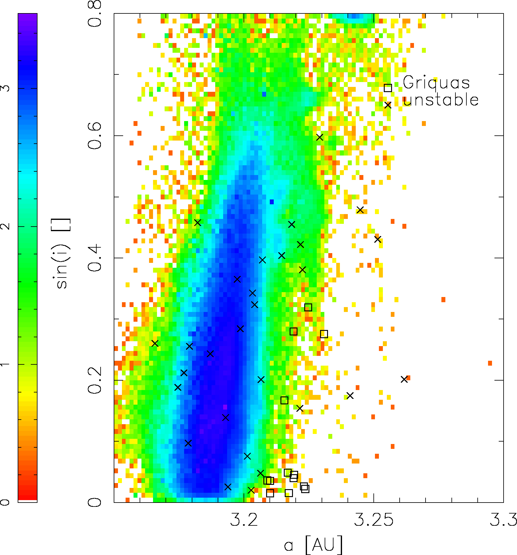
Thus we modified the previous plots in the following way:
- (i) TPs are plotted only during the interval of time, when they reside inside the J2/1 resonance (identified by the begining and the end of large oscillations of the semimajor axis around the center of the resonance at approximately 3.255 AU);
- (ii) the (a, e, sin(i)) space is divided to several parts: inclination lower or higher than 5 degrees and eccentricities lower or higher than 0.3 - the stable Zhongguos should then be compared with low-inclined and low-eccentricity orbits and unstable asteroids with high-inclined and high-eccentricity ones. Of course, one TP might enter different parts of the space during its orbital evolution.
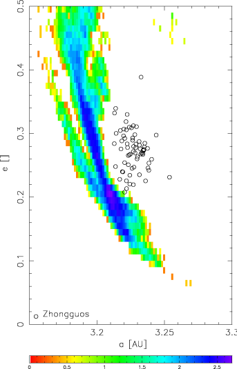
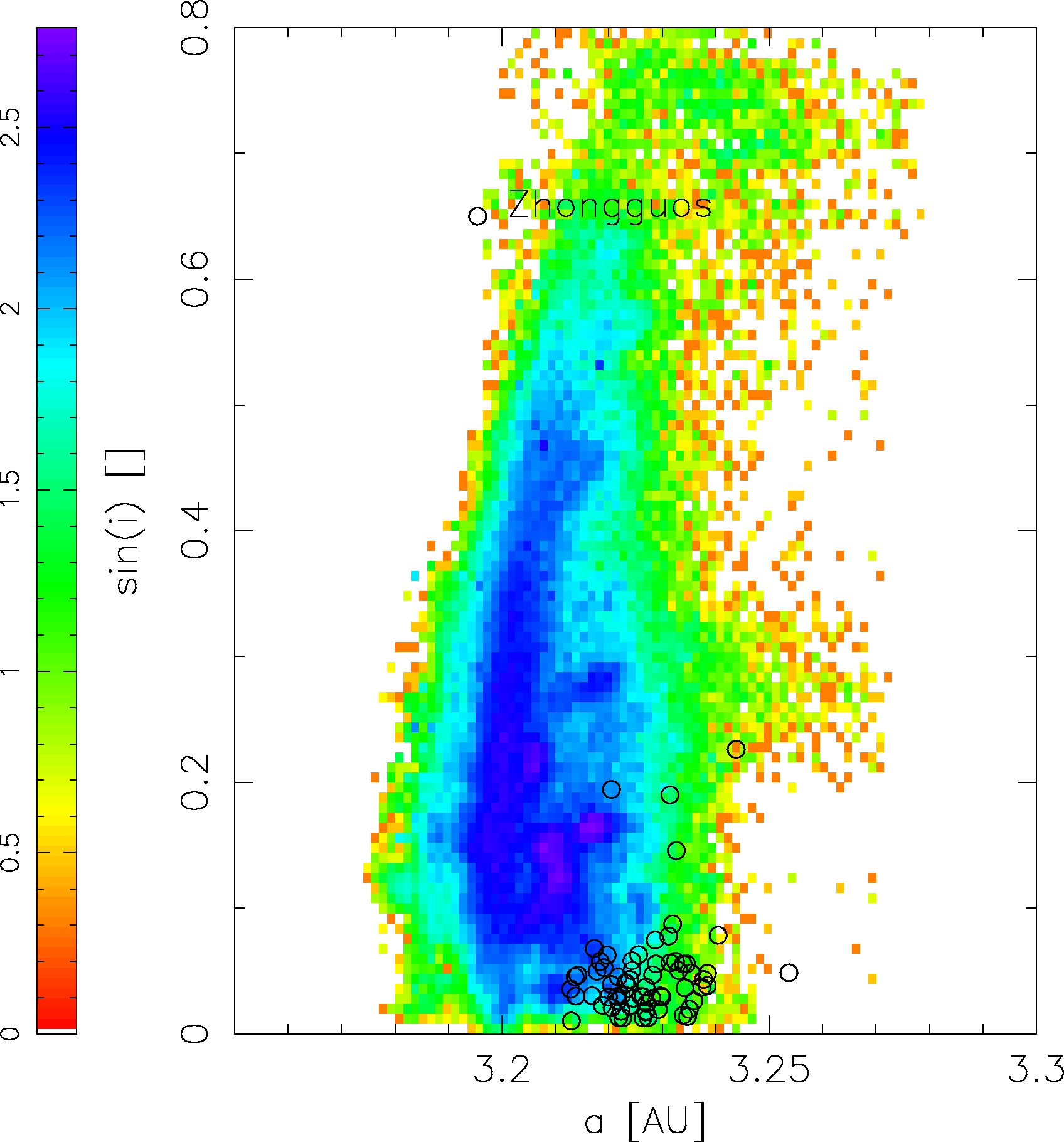
A comparsion of TPs orbits inside the J2/1 resonance, which fulfil the condition i < 5° and e < 0.3, with the observed population of Zhongguos:
 [ 300 DPI
| EPS ]
[ 300 DPI
| EPS ]
 [ 300 DPI
| EPS ]
[ 300 DPI
| EPS ]
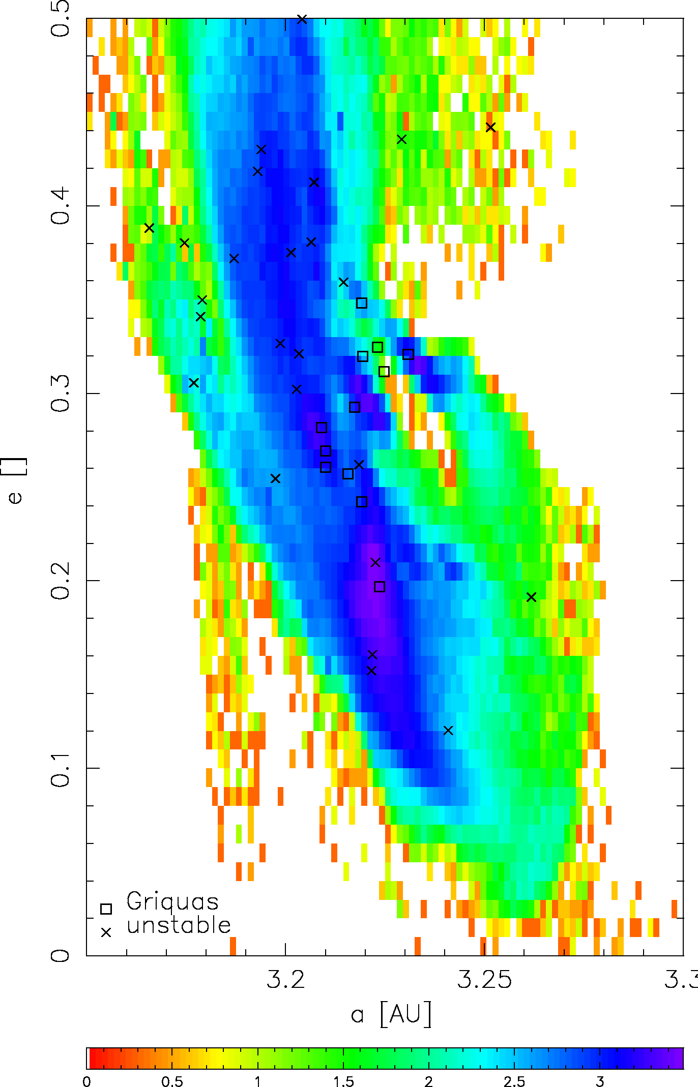
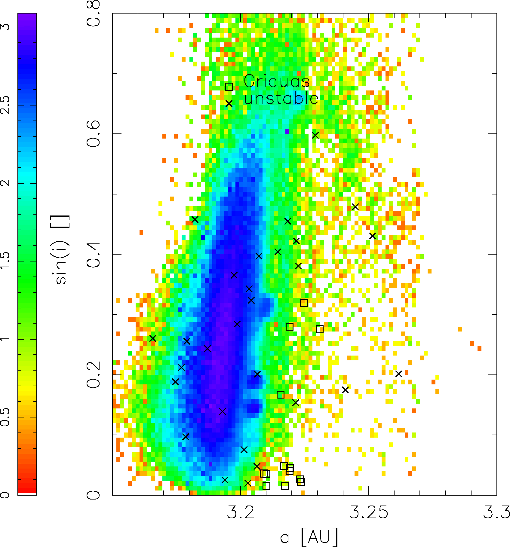
A similar comparsion of orbits inside the J2/1 resonance, which fulfil the condition i > 5° and e > 0.3, with the observed population of unstable asteroids:
 [ 300 DPI
| EPS ]
[ 300 DPI
| EPS ]
 [ 300 DPI
| EPS ]
[ 300 DPI
| EPS ]
To make things more sophisticated, we also provide:
- Three projections (a, e), (a, sin(i)) and
(e, sin(i)) on a surface of a cube and another two planes
slicing through the volume:
[TO COME SOON]
- 3-D plots with density isosurfaces probably may give the best insight to the situation. There is a single illuminated isosurface with a value of 1000 in the first figure and two isosurfaces (100 and 1000) in the second. (The animations are available in a higher resolution in AVI format.)
 [
[  [
[ With these results we would say that: (i) Zhongguos and Griquas are `missed' by the bulk of integrated orbits, while (ii) the 2/1 region occupied by the unstable asteroids may be well matched by the evolving orbits of integrated TPs. A deeper look on that is below.
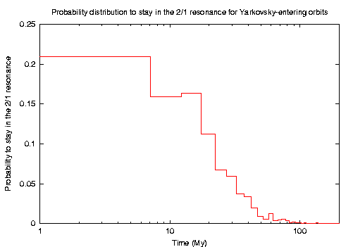
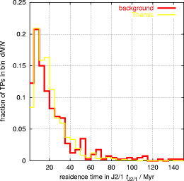
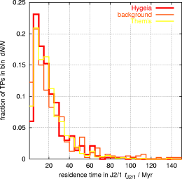
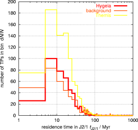
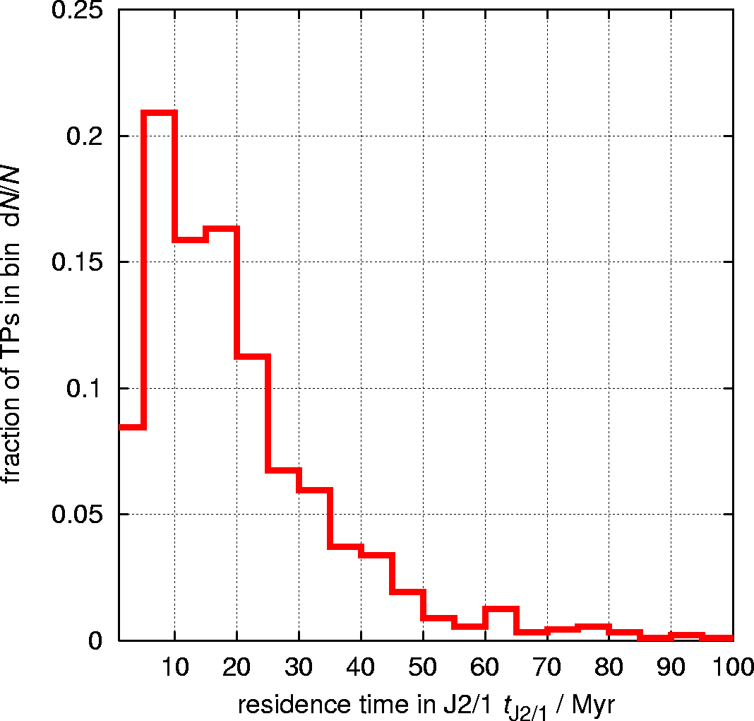
Another `diagnostics' is to compare (i) dynamical lifetime of the observed asteroids on unstable orbits inside the 2/1 resonance and (ii) residence time of our integrated orbits inside the 2/1 resonance. Here we also show the probability distribution of the total residence time in the 2/1 resonance for the integrated orbits:
 [ 300 DPI
| EPS ]
[ 300 DPI
| EPS ]
 [ 300 DPI
| EPS ]
[ 300 DPI
| EPS ]
 [ 300 DPI
| EPS ]
[ 300 DPI
| EPS ]
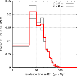
Data files: table of residence times, histograms of residence times and times of entry into the J2/1.
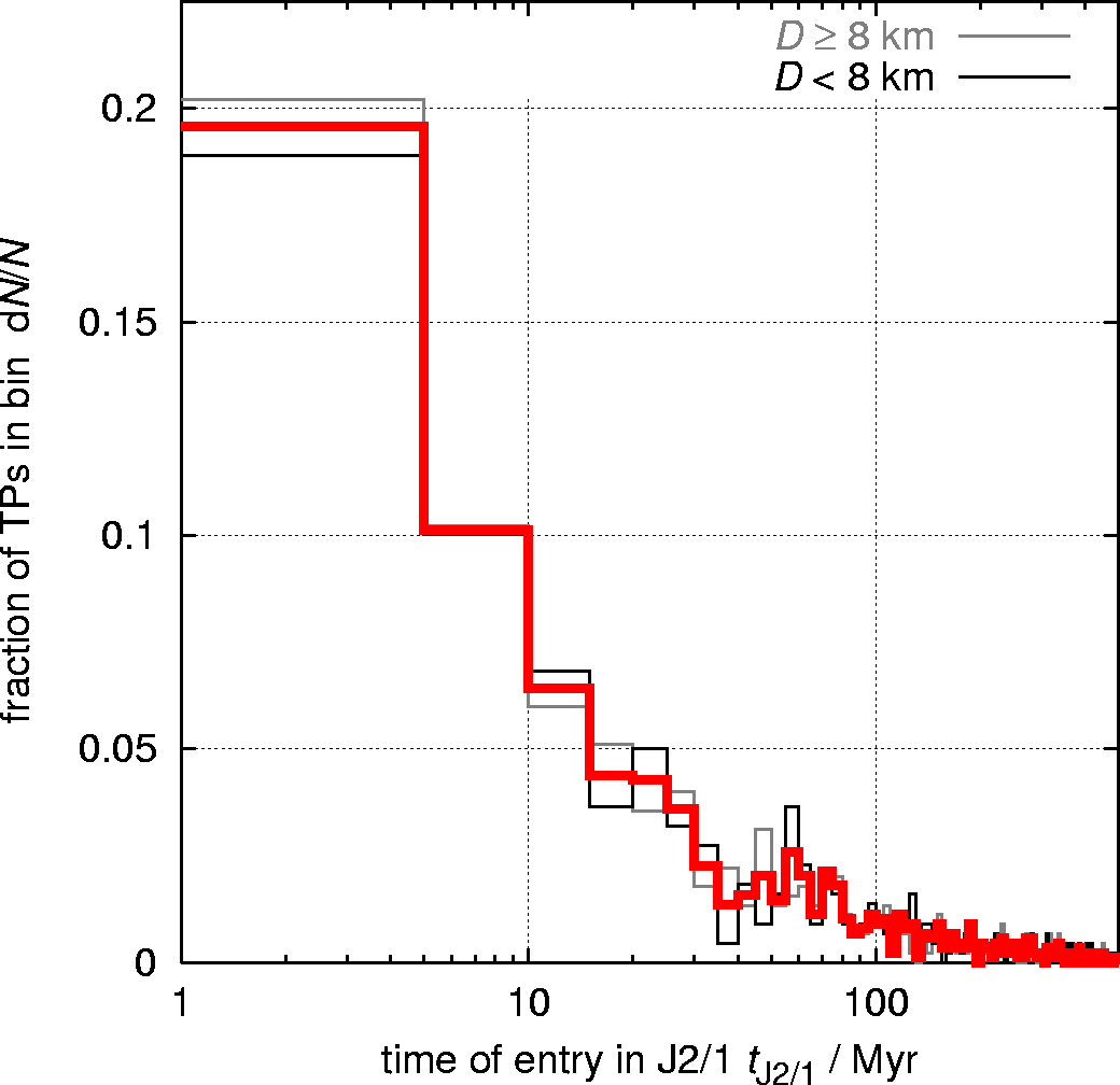
The histograms for asteroids >8 km in diameter: residence times, times of entry; and also <8 km: residence times, times of entry.
We note, a medium time to spend in the resonance is between 15-20 My, that matches very well a typical dynamical lifetime that characterises the unstable population of asteroids. We divided the integrated sample of asteroids into two groups, bodies larger than 8 km and bodies smaller than 8 km, and determined the residence time distributions separately for the two classes. The results were basically identical, as expected. This information is used below in the semianalytic model.
Oscillations of resonant elements and direct comparsion of TPs paths with cells, where observed asteroids reside.
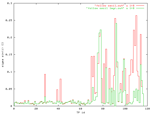
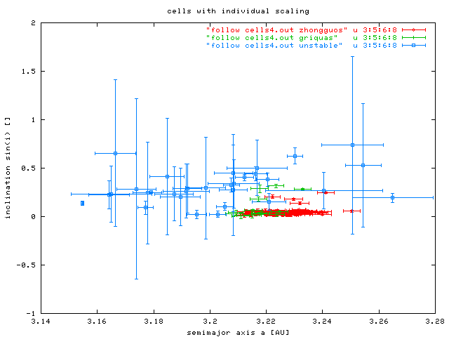
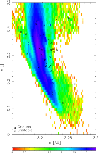
At first we have to characterize somewhat more deeply location of the observed asteroids inside the 2/1 resonance. Note that the resonant proper elements, that we compute, contain information about the fundamental variations of elements in the resonance (namely the ~ 400 y and ~ 20 ky cycles), but dynamics inside the resonance is intrinsically chaotic and even the resonant proper elements evolve on a long term. We thus need to practically measure this potential `wandering' of resonant a, e, sin(i) for observed members of Zhongguos, Griquas and unstable populations.
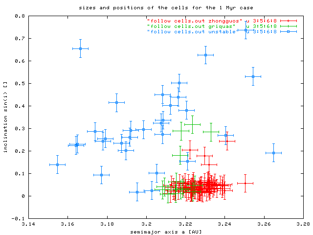
We found a good trade to integrate all observed asteroids inside the 2/1 resonance for 1 My and record their resonant proper elements. Those fill some region and we characterize it with: (i) center, and (ii) 1-sigma dispersion in a, e and sin(i). Here is the result:
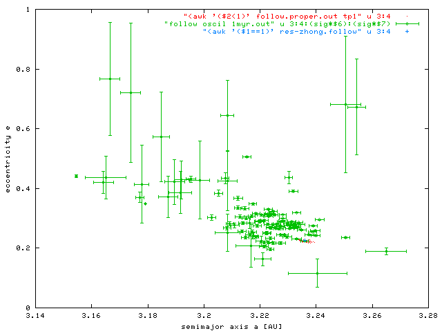
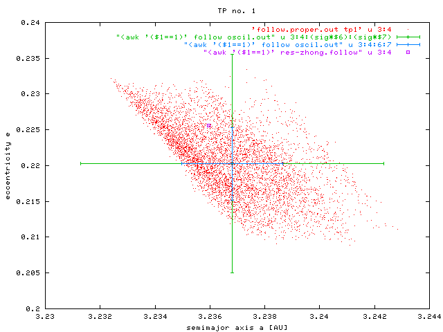
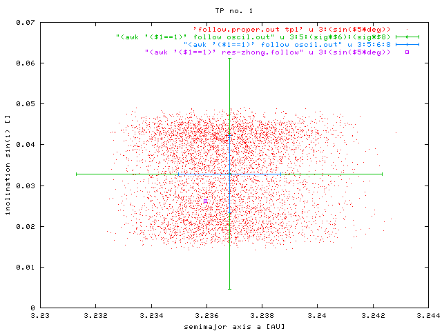
To see in little more detail our procedure look here at TP no. 1 (a Zhongguo-like asteroid): (i) resonance proper elements plotted in red colour, and (ii) our 1-My box shown by the cross. We show (a, e) and (a, sin(i)) projections and 1-sigma and 3-sigma dispersions (error-bars). In what follows we are going to choose 2-sigma as a compromise for purposes of scaling of individual cells.
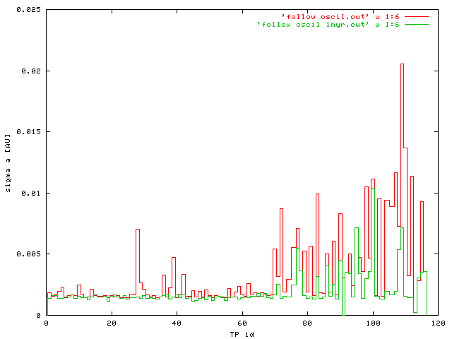
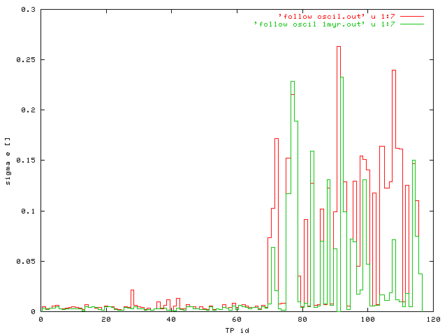
The amplitudes of oscillations ("1-sigma") in a, e, sin(i) as functions TP identification numbers. TPs no. 1-69 are Zhongguos, the rest is a "mixture" of Griquas and unstable population. We arbitrary chose some-sort-of mean values of oscillations as common sizes of fixed (a, e, sin(i)) cells: semimajor axis 0.004 AU, 0.02 in eccentricity and 0.04 in sine of inclination.
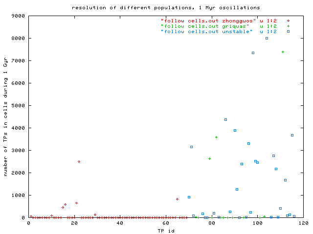
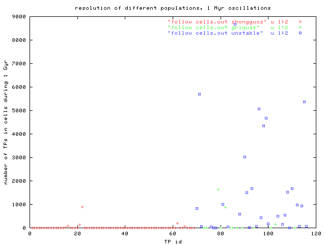
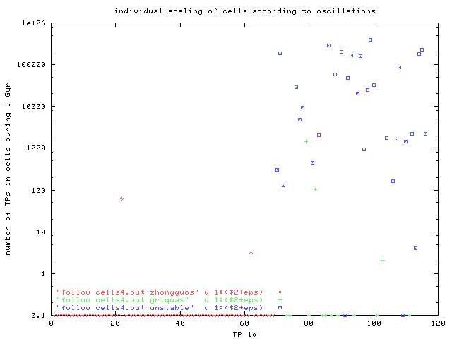
We are now ready to compare the distribution of our TPs with populations of observed asteroids. The main quantity, shown in the following figures, is the number of TPs that reside inside particular cells of the observed asteroids (defined above). To still see how results depend on the above determined size of the individual cells we also once take into accound fixed cell (averaged from all cases) for all asteroids.
The plots number of TPs vs. TPs id. number show, that practically only the cells of unstable population are attended by our TPs. The three observed populations could be distinguished by different colours. The only significant difference between fixed-size cells (the left figure) and individually scaled cells (the right figure) is the higher "number of TPs", what is, of course, caused by the larger oscillations of "unstables" and correspondingly larger size of their cells.
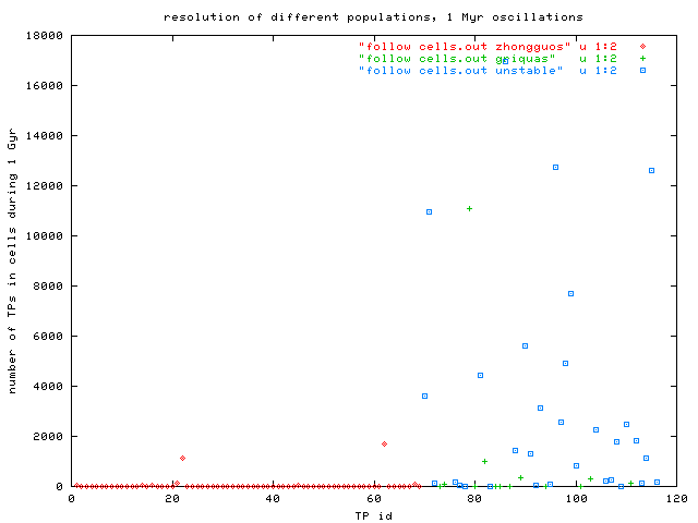
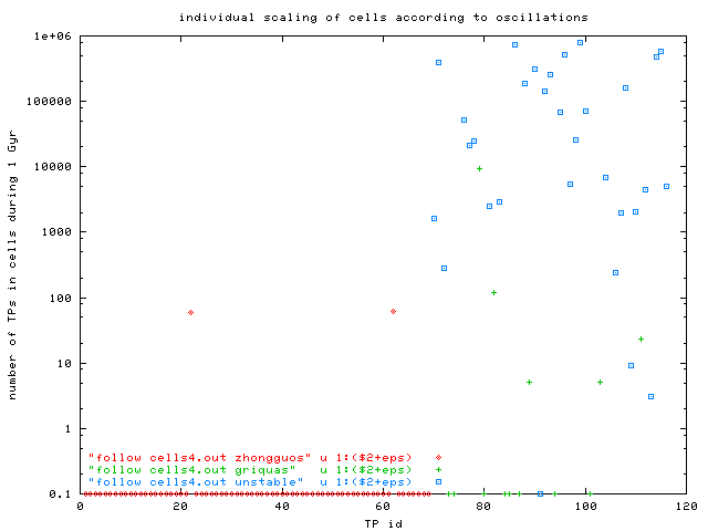
The sizes of cells are depicted in the following four plots. (The left-hand figures have fixed sizes, the right-hand not.)


The last four plots concerning this issue show the situation in 3-D space of either (resonant a, resonant e, number of TPs) or (resonant a, resonant sin(i), number of TPs). Note, that z-scale is logarithmic for the case of individial cell scaling.


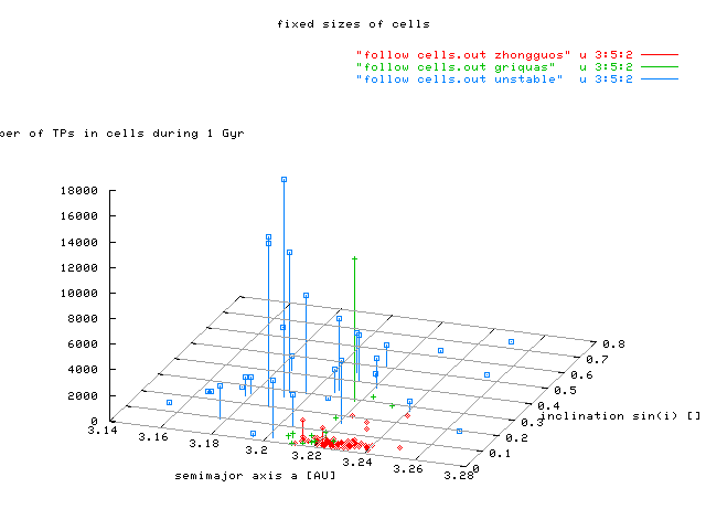

In conclusion: (i) most cells corresponding to the observed unstable asteroids, were frequently visited by our integrated TPs and are thus well compatible with assumption that the Yarkovsky delivery populates them; and (ii) Zhongguos are not visited at all, a few exceptional Griquas are visited, but majority of them is also outside the Yarkovsky fed flow of orbits.
Below we repeat our analysis in brief for the other two possible source regions of the unstable asteroids in 2/1: background asteroids and Hygiea family asteroids.
Background population as a source.
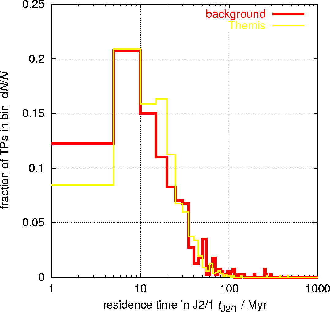
The distribution of residence times in the J2/1 resonance of the background population is very similar to the TPs originated in the Themis family (the first plot is in linear scale and the second in logarithmic scale):
 [ 300 DPI
| EPS ]
[ 300 DPI
| EPS ]
 [ 300 DPI
| EPS ]
[ 300 DPI
| EPS ]
Data files: table of residence times, histograms of residence times and times of entry into the J2/1.
A comparsion of TPs orbits inside the J2/1 resonance, which fulfil the condition i < 5° and e < 0.3, with the observed population of Zhongguos:
 [ 300 DPI
| EPS ]
[ 300 DPI
| EPS ]
 [ 300 DPI
| EPS ]
[ 300 DPI
| EPS ]
A similar comparsion of orbits inside the J2/1 resonance, which fulfil the condition i > 5° and e > 0.3, with the observed population of unstable asteroids:
 [ 300 DPI
| EPS ]
[ 300 DPI
| EPS ]
 [ 300 DPI
| EPS ]
[ 300 DPI
| EPS ]
The plots number of TPs vs. TPs id. number: only unstable asteroids are visited by out TPs.

Hygiea family as a source.
Again, the distribution of residence times in the J2/1 resonance of the Hygiea family is quite similar to the TPs originated in the Themis family:
 [ 300 DPI
| EPS ]
[ 300 DPI
| EPS ]
 [ 300 DPI
| EPS ]
[ 300 DPI
| EPS ]
Data files: table of residence times, histograms of residence times and times of entry into the J2/1.
A comparsion of TPs orbits inside the J2/1 resonance, which fulfil the condition i < 5° and e < 0.3, with the observed population of Zhongguos:
 [ 300 DPI
| EPS ]
[ 300 DPI
| EPS ]
 [ 300 DPI
| EPS ]
[ 300 DPI
| EPS ]
A similar comparsion of orbits inside the J2/1 resonance, which fulfil the condition i > 5° and e > 0.3, with the observed population of unstable asteroids:
 [ 300 DPI
| EPS ]
[ 300 DPI
| EPS ]
 [ 300 DPI
| EPS ]
[ 300 DPI
| EPS ]
The plots number of TPs vs. TPs id. number: again, only unstable asteroids are visited by our TPs.
Semianalytic steady-state model.
In order to quantify the absolute number of asteroids residing on the unstable orbits in 2/1 resonance we use a semianalytic model developed by Morby and David V. for NEAs [Ref]. Its formulation is basically the same as in this earlier work and I have just a few comments before discussing results.
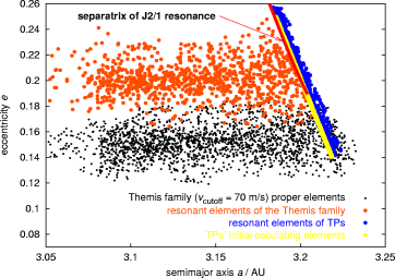
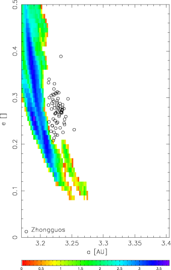
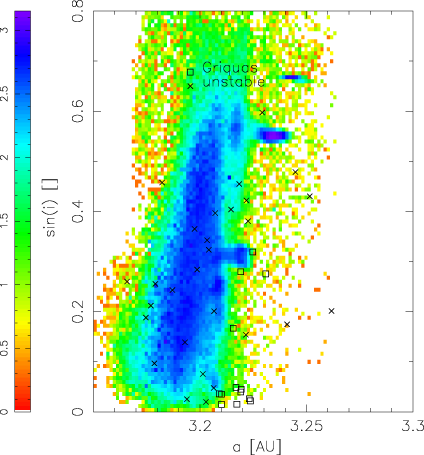
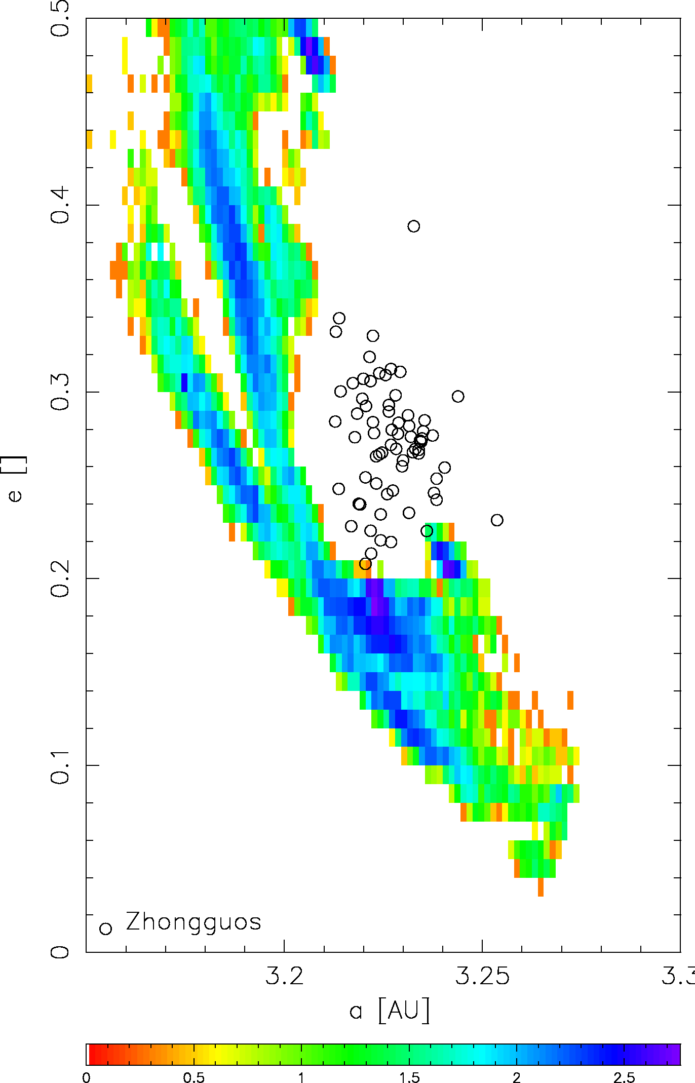
2/1 resonance border. I use an approximate formula e(a) = 10.818551 - 3.3183427 * a to determine border of the 2/1 resonance (see the magenta line in the figure below). This is certainly rough, but I guess OK for sake for the method we use.
Source population. To set things simple, I consider a database of analytic proper elements from AstDyS (the `famous' files allnum.pro and ufitobs.pro). A question may be why not using the synthetic proper elements, but finally I believe the difference would not be that great; the analytic elements give us information about more objects: something like 132000 asteroids in total, and about 13000 for Themis and Hygiea families and the background population with a > 3.1 AU. Here I show their projections into the proper element planes (a,e) and (a,sin I).
|
|
|
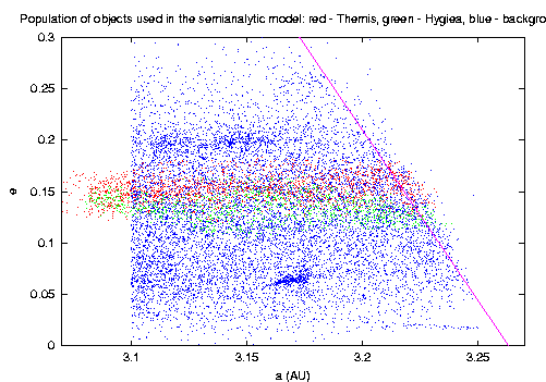
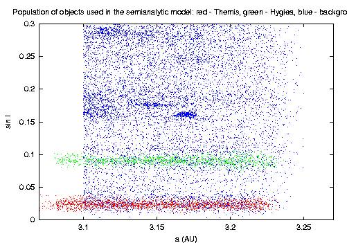
A few things are certainly remarkable here: (i) the sharp cutoff at 3.1 AU is obviously `arbitrary' and does not affect our results (see also below), (ii) note the background population of asteroids (blue) really dominates in number the family asteroids (including Themis, red), (iii) Themis is very sharp structure in the inclination, and majority of objects below 2/1 resonance do not have that low value of I.
In our approach we manipulate each of the objects in the source population `individually'; initially they occupy (a,e,sin I) locations of the observed bodies (as shown in the figures above), but as I explain below I consider a population consisting of quite more test bodies. Some of them have been assigned the same (a,e,sin I) initial positions, but they undergo different evolution due to the Yarkovsky (and YORP) effects. I keep track of the initial subpopulation for a particular body (background, Themis or Hygiea). Initially, spin axes are randomly oriented in space.
Another issue is to assign a particular size distribution of the initial population that is going to be `manipulated' by the code. In order to better pick the slope of the size distribution near ~ 10 km I do not use the real populations (that certainly start to suffer from incompleteness problems there) but I use `fake' power-law populations generated by the following procedure:
- Background population: (i) sample of asteroids with sizes larger than 25 km is assumed complete and taken as it is observed; (ii) below 25 km size I fit the population with a power law of exponent -2.62 (cumulative distribution), and (iii) in order not to exagerate number of small bodies I assume a change of the exponent to -2.5 below 10 km size. This is a value for collisionally relaxed population; we shall see below that the result does not critically depend on assumption of this exponent at small sizes.
- Themis population: (i) down to 25 km the population is assumed complete as for the background population, (ii) between 20 and 25 km size the population is fitted with a power law of exponent -2.62, and (iii) below 20 km I `tie' the distribution to the background so that the bias factor in each size cells are the same for the two populations. This assumption is consistent with procedure in Morby et al. [Ref].
- Hygiea population: (i) down to 25 km the population is assumed complete as for the background population, (ii) between 20 and 25 km size the population is fitted with a power law of exponent -4.2, and (iii) below 20 km I `tie' the distribution to the background so that the bias factor in each size cells are the same for the two populations. This assumption is consistent with procedure in Morby et al. [Ref].
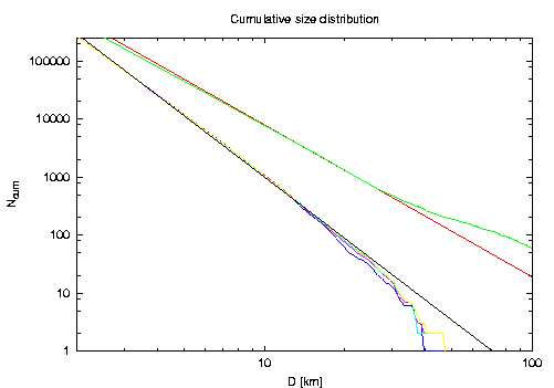
Here is the comparison of the real and fake populations:
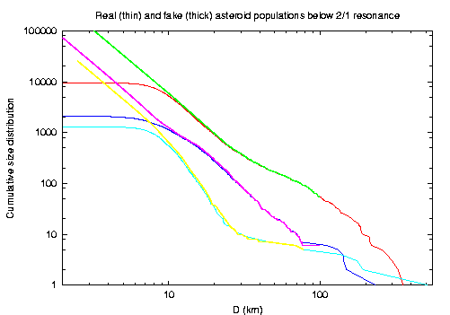
A few comments are appropriate: (i) I disregard large asteroids (> 100 km size, say) in all populations, in particular the background and Hygiea family; this is however fine, since we anyway do not expect they would move by Yark effect and reach the 2/1 resonance; and, what is more relevant, (ii) at 9 km the fake populations (green, magenta and yellow) contain more asteroids than the observed populations. The effect (ii) is likely real and reflects observational incompleteness. Note however that we apparently do not exagerate the >9 km population, making it larger than the observed one by a factor of ~ 6690/6350 ~ 1.05 for the background population; with the adopted procedure explained above that ratio stays the same also for the other two populations.
Yark and YORP modelling. Now with this initial population set, I start running the code; the final time is 4 Gy and a timestep is 0.5 My. The basic features are (i) evolution in semimajor axis due to the Yarkovsky effect [Ref], and (ii) obliquity-spin-rate evolution due to the YORP effect [Ref]. As far as the Yark effect is concerned, I consider bulk density of 1.7 g/cm3 and thermal parameters guessed for hydrated surface (a mixture of ice and rocks, say). The usual formulae of the linearised theory are used with fundamental dependence on size (such as 1/size) and obliquity; diurnal effect typically dominates. YORP setting profits from a few, still unpublished, improvements we have with David Capek, notably YORP torques computed for bodies with finite surface thermal conductivity. I do include collisional reorientations of the spin axes according to the formula (8) in Morby's and David V.'s NEAs paper [Ref].
I also recall the basic feature of the model, already explained in detail in our NEA paper [Ref], namely we assume a steady state-situation. In reality, this may not be exactly true, but it is definitely the best starting assumption we can do. It largely simplifies modelling, because we do not need to care about details of collisional dynamics. In order to force the system to be in long-term steady-state, with only some fluctuations, we play the following trick: when some asteroid enters the 2/1 resonance, it is recorded as `resonant', but another body is put in the source population to replace it (actually we pick randomly one of the initial objects, keeping however the size of the body that entered the resonance). In fact, the procedure is still little more tricky. I use the information how long the numerically integrated orbits (above) typically stay in the resonance and leave the body in the resonant buffer for a time according to the computed probability distribution. I record the interval of time the body presumably stayed in the resonance and only then would replace it by a new object in the source population. The information about residence in the 2/1 is then used to evaluate the expected steady-state population of asteroids inside 2/1.
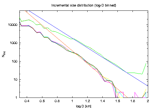
Results. I start commenting on `the nominal job' where nominal strengths of the Yarkovsky and YORP effects were included, collisional reorientations taken into account but collisional disruptions disregarded. I recall that at the output of the simulation I get a listing recording that a given asteroid of size D reached the 2/1 resonance at a time t1 and was scattered out at a time t2. First, I analyse the size distribution of the modelled resonant population. To get a fair sample, for which I would be able to determine a reasonable slope of the size distribution, I collect asteroids that resided (passed through) the resonance during some, long enough, timespan -- I tried 2 Gy. To see how much the result depends on the choice of the particular `window', I use a running window in between 0.5-2.5 Gy, 1-3 Gy, 1.5-3.5 Gy and 2-4 Gy. Doing that I certainly obtain a fake population of objects in 2/1, far too large as compared to a population observed at any particular time, but I hope to obtain a reasonable mean of the expected size distribution of the resonant population. The results are shown in the next two figures: (i) on the left, I give the `conventional' cumulative size distribution, and (ii) on the right I give incremental size distribution but binned in log-D bins; this means that the exponents in both cases are (should be) the same and I can compare the two methods to estimating/fitting the exponent of the resonant population.
|
|
|
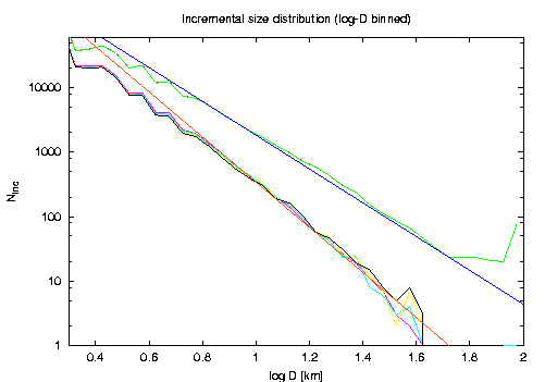
The upper distribution is Themis, and its power-law fit with exponent -2.6, and the lower distribution is the 2/1 population of unstable asteroids with its power-law fit having an exponent of -3.50. The latter value is pretty close to the observed value derived above. We obviously anticipated a change in the exponent due to the size-dependence of the Yark effect (`makes -1 effect') and the YORP effect causes a little `softening'.
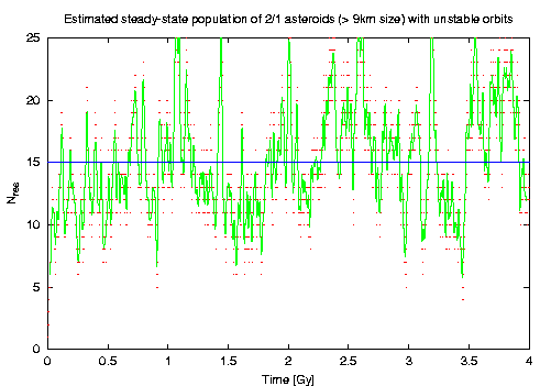
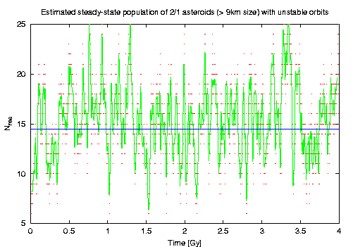
Now we care about the expected population of the Yarkovsky-transported unstable 2/1 asteroids quantitatively. This is done by just looking at each timestep how many objects reside in 2/1. The corresponding plot, showing number of asteroids D>9 km, is here:
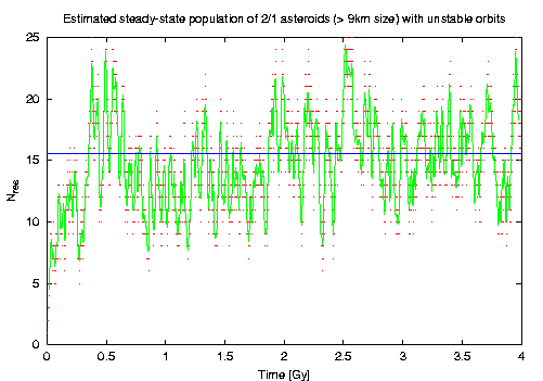
(red dots are raw data and green line is a filtered representation). Here also things seem to go right: we would expect something like 15.5 asteroids larger than 9 km on the unstable orbits. This is fairly close to the observed population of 14 of them!
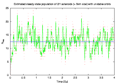
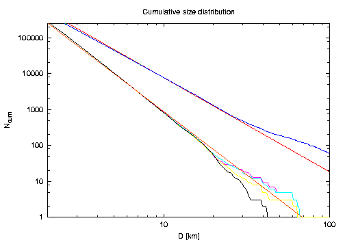
Additional results and tests. Next we check how robust is the above solution by varying several of free parameters. First we care about the role of the `artificial cut' of the background population at 3.1 AU; in fact, we anticipate it should not harm, because changing this limit (e.g. increasing to 3.13 AU as in the test below) we make the population smaller in quantitative terms, but on the other hand it is overall closer to the 2/1 resonance so that the bodies would more easily reach the resonance. Obviously, this assumes that the size distribution does not change severely as we go closer to the resonance (perhaps likely the case unless very close to the resonance). I thus did a test and placed the lower limit of the background population at 3.13 AU; otherwise the size-distribution characteristics of the populations were as in the previous run (i.e. shallowed populations near 10 km threshold). Results confirmed the guess and nothing changed.
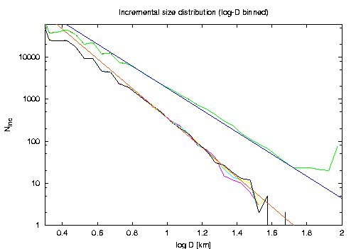
I also checked that the result little depends on our assumption about the second slope (below 10 km size) of the size distribution of the background population (taken -2.5 above). It is however known (REFS) that overall main belt population seem to have quite shallower local exponent of the size distribution in the range 1 - 10 km. We thus made the similar simulation as above but considering an exponent -2 below 10 km in the background population; both Themis and Hygiea populations of small asteroids is again tied to the background population with the argument of the same observational bias. With these parameters the > 9 km fake population is larger than the observed population by only a factor of 1.004 (thus basically the same). Results are shown here (note the shallower end at smaller sizes):
|
|
|

We note that nothing serious has changed: (i) flux in 2/1 got little more fluctuated, but the average stays around 15 asteroids on the unstable orbits, and (ii) the slope of -3.50 in their size distribution still fits the same.
Next, I included also collisional disruptions. This is done in a similar way as in Morby and Vok (2003) model [Ref] for feeding of the NEA population. Notably, we assumed a collisional lifetime of 16.8 \sqrt{R} My (R is radius in metres) and at each timespet of the simulation we check statistical possibility of a disruption. When a body is assumed disrupted, it is replaced with a randomly chosen object of the same size feom the initial population (with rotation reset). In that way we again enforce the steady-state situation. With this change, we run the code again and obtained the following result:
|
|
|
Again, results are little changed: I only modified the exponent of the resonant population to -3.54 as it looks little steeper than before.
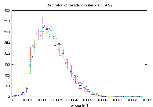
Well so far it looks great, though there is one hidden caveat that I started to dig now -- I keep the previous text for `continuity'. I consider the last, or the last but one, simulation, and for sake of interest I looked at distribution of the rotation rate and obliquities of the main-belt population asteroids at some (arbitrary though) times -- say 0, 1, 2, 3 and 4 Gy. Since our `target population' of bodies are those with size > 9 km, I used only those. As far as their rotation rate distribution concerns, nothing `really disturbing', I got something like in the following plot:
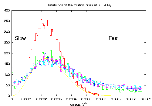
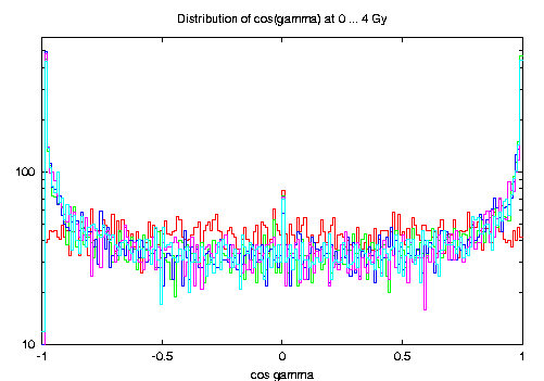
the red histogram is a bit `arbitrary' initial population that settles into distribution shown by the other histograms. Compared to the Maxwellian distribution (yellow), there is an overabundance of slow and fast rotators, certainly due to the YORP effect. For what we know, large asteroids (like > 40 km) follow Maxwellian distribution, but who knows what is the exact distribution of the exterior-main-belt asteroids with sizes about > 10 km. However, `more disturbing' was to see distribution of their obliquities (actually cos(obliquity)):

The evolved distributions, all curves except the initial isotropic in red, show many spins pushed by YORP to the extreme values cos(obliquity)=+-1; actually from ~8300 asteroids larger than 9 km, some 2/3 were in the four most extreme bins. Again, we do not have much idea what is the real distribution, but this seems stretching too much. So I looked around what might be changed in the model. First, certainly I may decrease strength of the YORP effect, but after `the Nature paper' I tend to have some degree of confidence to what we predict. There is another area where perhaps our modelling is more vague, namely collisional lifetimes and reorientation timescales. I used our old estimates (actually done once upon a time by Paolo Farinella), but who knows how exactly the material strength varies to the C-types in the studied region of the belt, how projectiles transmit angular momentum into C-type targets etc. So I played the `stupid' game to multiply the nominal formulae for collisional lifetime and reorientation timescale -- eqs. (9) [with A=16.8 My and alpha=0.5] and (10) in Morby and David V. [Ref] -- by some arbitrary scaling factors c1 [for the collisional lifetime] and c2 [for the reorientation timescale]. In the next panel I summarize results for c1=1,0.1 and c2=1,0.1 [obviously 1,1 case is the previously discussed, nominal solution].
| c1=1 | c1=0.1 | c2=1 | 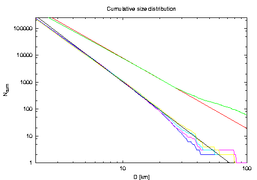 2/1 population: SD exponent = -3.50, mean population = 15.5 |
  2/1 population: SD exponent = -3.52, mean population = 12.5 |
c2=0.1 | 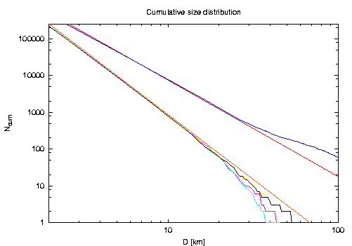 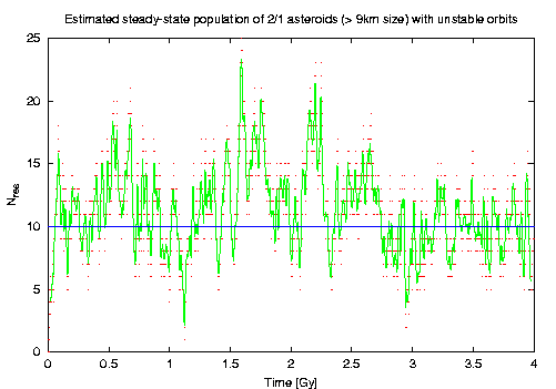 2/1 population: SD exponent = -3.52, mean population = 10 |
  2/1 population: SD exponent = -3.52, mean population = 12.5 |
and here is the check on the obliquity distribution of the >9 km main-belt asteroids:
| c1=1 | c1=0.1 | c2=1 | |
 |
c2=0.1 | 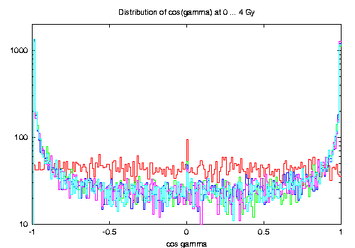 |
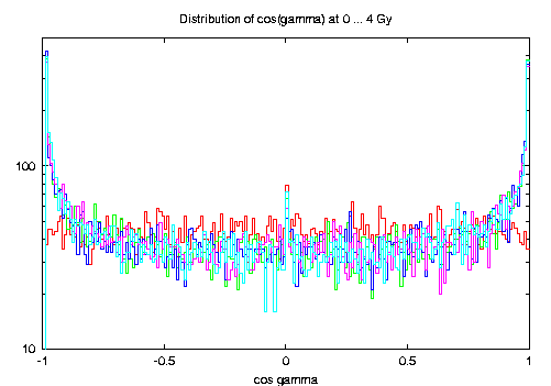 |
Well, cases like c1=0.1 [might be ok due to C-type smaller strength compared to Paolo's lifetime formula for S-types] and c2=0.1 [who knows :] look already reasonably well and still yield something like 12 asteroids in mean delivered onto the unstable orbits in the 2/1 resonance. Also the distribution of the rotation rates look quite more Maxwellian for the c1=0.1 and c2=0.1 case as seen from the following figure: